Programming tools in data science > Tutorials > Project-oriented workflow

Project-oriented workflow

It’s like agreeing that we will all drive on the left or the right. A hallmark of civilization is following conventions that constrain your behavior a little, in the name of public safety. Jenny Bryan

Introduction

In this tutorial we will learn key aspects of making a good research project:

reproducible
portable
self-contained

In data science context, reproducibility means that the whole analysis can be recreated (or repeated) from the fresh start and raw data and get exactly the same results. It means, for instance, that if the analysis involves generating random numbers, then one has to set a seed (an initial state of a random generator) to obtain the same random split each time. Ideally, everyone should also have an access to data and software to replicate your analysis (it is not always the case, since data can be private).

Portability means that regardless the operating system or a computer, for minimal given prerequisites, the project should work. For instance, if the project uses a particular package that works only on Windows, then it is not portable. The project is also not considered as portable, if it utilizes a particular computer settings, such as absolute paths instead of relative to your project folder (e.g., when reading the data or saving plots to files). Normally, you should be able to run the code on your collaborator’s machine without changing any lines in scripts.

We call a project self-contained, when you have everything you need at hand (i.e., in the folder of your project) and your porject does not affect anything it did not create. The project should not use a function, which you created in the other project five years ago – it is very likely that no one else has this function. Further, if you need, for instance, to save a processed data, then it should be saved separately, and not overwrite the raw data.

Why this is a big deal? First off, it gives more credibility to the research, because it can be verified and validated by a third party. Further, keeping the flow of analysis reproducible, portable and self-contained makes it easier to extend.

There are no clear boundaries between these three properties, they are very close in meaning, and often overlap. As a consequence, techniques and practice we consider further improve all of them, rather than focusing on a particular one.

map

Even if it might look like a yet another git / RStudio tutorial, this is a list of my recommendations based on my own experience and various posts.

Project folder structure

The size of the project increases exponentially. A project started as a harmless code snippet can easily pile up into a huge snowball of over hundred files with unstructured folder tree. To avoid this, it is important do define the folder structure before stepping into analyses. Depending whether the project is a package or a case study, its skeleton differs significantly.

The folder structure of R packages is a subject to a regulation of community (CRAN and Bioconductor). It is well-defined and can be explored in R packages book, therefore, I skip it in this tutorial.

In contrast to R packages, there is no a single right folder structure for analysis projects. Below, I present a simple yet extensible folder structure for data analysis project, based on several references that cover this issue.

name_of_project/
|-  data
|   |-  raw
|   |-  processed
|-  figures
|-  reports
|-  results
|-  scripts
|   |-  deprecated
|-  .gitignore
|-  name_of_project.Rproj
|-  README.md

The parent folder that will contain all project’s subfolders should have the same name as your project. Pick a good one. Spending an extra 5 minutes will save you from regrets in the future. The name should be short, concise, written in lower-case, and not contain any special symbols. One can apply similar strategies as for naming packages.

The folder data typically contains two subfolders, namely, raw and processed. The content of raw directory is data files of any kind, such as .csv, SAS, Excel, text and database files, etc. The content of this folder is read only, so that no scripts should change the original files or create new ones. For this purpose the processed directory is used: all processed, cleaned, and tidied datasets are saved here. It is a good practice to save files in R format, rather than in .csv, since the former one is a more efficient way of storing data (both in terms of space and time of reading/writing). The preference is given to .rds files over .RData (see why in Content of R files section). Again, files should have representative names (merged_calls.rds vs dataset_1.rds). Note that it should be possible to regenerate those datasets from your scripts. In other words, if you remove all files from this folder, it must be possible to restore all of them by executing your scripts that use only the data from raw.

The folder figures is the place where you may store plots, diagrams and other figures. There is not much to say about it. Common extensions of such files are .eps, .png, .pdf, etc. Again, file names in the folder should be meaningful (the name img1.png does not represent anything).

All reports live in directory with the corresponding name reports. These reports can be of any formats, such as LaTeX, Markdown, R Markdown, Jupyter Notebooks, etc. Currently, more and more people prefer rich documents with text and executable code to LaTeX and friends.

Not all output object of the analysis are data files. For example, you have calibrated and fitted your deep learning network to the data, which took about an hour. Of course, it would be painful to retrain the model each time you run the script, and you want to save this model. Then, it is reasonable to save it in results with .rmd extension.

Perhaps the first by importance folder is scripts. There you keep all your R scripts and codes. That is the exact place to use prefix numbers, if files should be run in a particular order (see previous tutorial). If you have files in other scripted languages (e.g., Python), it better to locate them in this folder as well. There is also an important subfolder called depricated. Whenever you want to remove one or the other script, it is a good practice to move it to depricated at first iteration, and only they delete. The script you want to remove can contain functions or analysis used by other collaborators. Moving it firstly to depricated ensures that the file is not used by other collaborators.

There are three important files in the project folder: .gitignore, name_of_project.Rproj, and README.md. The file .gitignore lists files that won’t be added to Git system: LaTeX or C build artifacts, system files, very large files, or files generated for particular cases. Further, the name_of_project.Rproj contains options and meta-data of the project: encoding, the number of spaces used for indentation, whether or not to restore a workspace with launch, etc. The README.md briefly describes all high-level information about the project, like an abstract of a paper.

The proposed folder structure is far from being exhaustive. You might need to introduce other folders, such as paper (where .tex version of a paper lives), sources ( a place for your compiled code here, e.g. C++), references, presentations, NEWS.md, TODO.md, etc. At the same time, keeping an empty folders could be misleading, and it is better to remove them (unless you are planning to store anything in them in the future).

Several R packages, namely ProjectTemplate, template, and template are dedicated to project structures. Also it is possible to construct a project tree by forking manuscriptPackage or sample-r-project repositories (repo for short). Using a package or forking a repo allow for automated structure generation, but at the same time introduce many redundant and unnecessary folders and files.

Finally, some scientists believe that all R projects should be in a shape of a package. Indeed, one can store data in \data, R scripts in \R, documentation in \man, and the paper \vignette. The nice thing about it that anyone familiar with an R package structure can immediately grasp where each type of a file located. On the other hand, the structure of R packages is tailored to serve its purpose – make a coherent tool for data scientists and not to produce a data product: there is no distinction between functions definitions and applications, no proper place for reports, and finally there are no place for other script languages that you can use (e.g, Bash, Python, etc.).

Content of R files

While there are no rules how to organize your R code, there are several dos and don’ts that most of the time are not tough explicitly. I cover them below:

Do not use the function install.packages() inside your scripts. You are not suppose to (re)install packages each time when you run your files. By default it is normally assumed that all packages that are used by a script are already installed.

If there are many of them to install, it is better to create a file configure.R, that will install all packages:
```
pkgs <- c("ggplot2", "plyr")
install.packages(pkgs)
```
The snippet above profits from the fact that install.packages() is a vectorized function. Anyway, most of the time, install.packages() is suppose to be called from the console, and not from the script.
Do not use the function require(), unless it is a conscious choice. In contrast to library(), require() does not throw an error (only a warning) if the package is not installed.

Use a character representation of the package name.

# Good 
library("ggplot2")
    
# Bad
library(ggplot2)

Load only those packages that are actually used in the script. Load packages at the beginning of the script.
Do not use rm(list = ls()) that erase your global environment. First, it could delete accidentally the precious heavy long-time-to-build object. Second, it gives an illusion of the fresh start of R.
Do not use setwd("/Users/irudnyts/path/that/only/I/have"). It is very unlikely that someone except you will have the same path to the project. Instead, use a package here and relative paths. The package here automatically recognizes the path to the project, and starts from there:
```
# Good
library("here")
    
cars <- read.csv(file = here("data", "raw", "cars.csv"))
    
# Bad
setwd("/Users/irudnyts/path/that/only/I/have/data/raw")
cars <- read.csv(file = "cars.csv")
```
If your script involves random generation, then set a seed by set.seed() function to get the same random split each time:
```
# Good 
set.seed(1991)
x <- rnorm(100)
    
# Bad 
x <- rnorm(100)
```

Do not repeat yourself (DRY). In R context it means the following: if the code repeated more than to times, you had better wrap it into a function.

# Better
fix_missing <- function(x) {
    x[x == -99] <- NA
    x
}
df[] <- lapply(df, fix_missing)
    
# Bad
df$a[df$a == -99] <- NA
df$b[df$b == -99] <- NA
df$c[df$c == -98] <- NA
df$d[df$d == -99] <- NA
df$e[df$e == -99] <- NA
df$f[df$g == -99] <- NA

Separate function definitions from their applications.
Use saveRDS() instead of save():

save() saves the objects and their names together in the same file; saveRDS() only saves the value of a single object (its name is dropped).

load() loads the file saved by save(), and creates the objects with the saved names silently (if you happen to have objects in your current environment with the same names, these objects will be overridden); readRDS() only loads the value, and you have to assign the value to a variable. Yihui Xie

Inizializing a new data analysis project

Disclaimer: the procedure below can be done in different ways. This particular way is no better than the others, but from author opinion has the most logical flow.

Prerequisites:

Installed and configured Git
Installed R and RStudio
Existing account in Github

Steps:

Pick a good name (e.g., beer).
In RStudio create a project:
- Navigate to File -> New project…
- Select New Directory
- Select New project (unless you are developing a package or a ShinyApp)
- Insert your picked name into Directory name
- Check Create a git repository

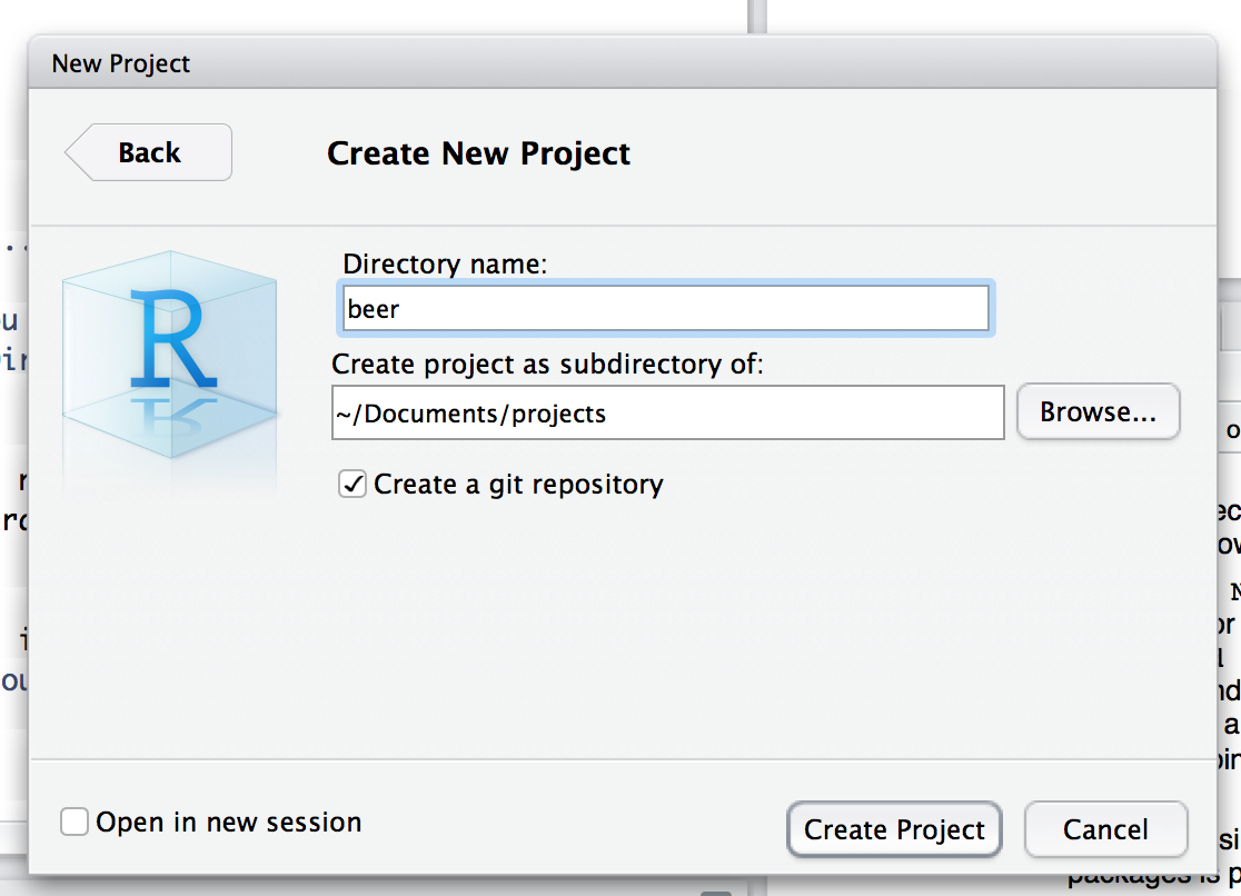
This creates a folder with the name of the project, initialize a local git repo, generate an .Rproj file, and a .gitignore file.

Add a file structure as discussed in section, that is folder data (with raw and processed subfolders), figures, etc.
Create a README.md file.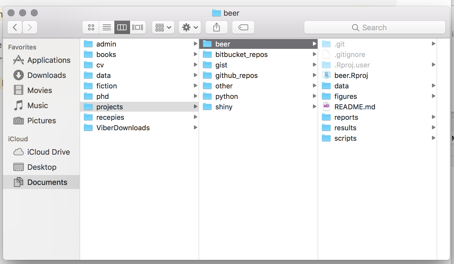
Launch Terminal and navigate your working directory (of Terminal, not R) to your project folder by, for instance, cd /Users/irudnyts/Documents/projects/beer.
Record changes by git add --all and commit by git commit -m "Create a folder structure of the project.". Traditionally the message of the first commit is simple "First commit.", but I prefer to write something more conscious, like "Create a folder structure of the project.".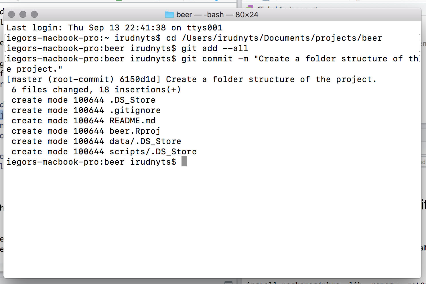

Now all you changes are recoreded locally.

Note also that Git does not record empty folders.
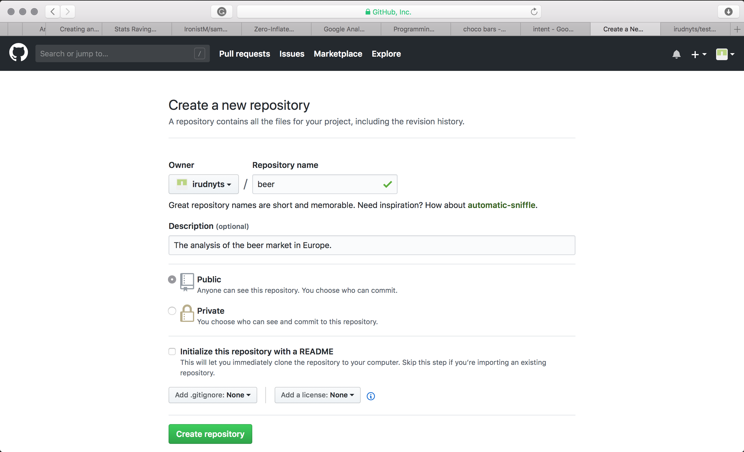
Create a new repo in GitHub (the same procedure holds for Bitbucket and Gitlab):
- Fill in Repository name with the same name as your project.
- Fill in Description with one line that briefly explains the intent of the project and ends with full stop.
- (Check Private for homeworks).
- Hit Create repository.
Connect your local repo to your Github repo by
```
git remote add origin git@github.com:irudnyts/beer.git
git push -u origin master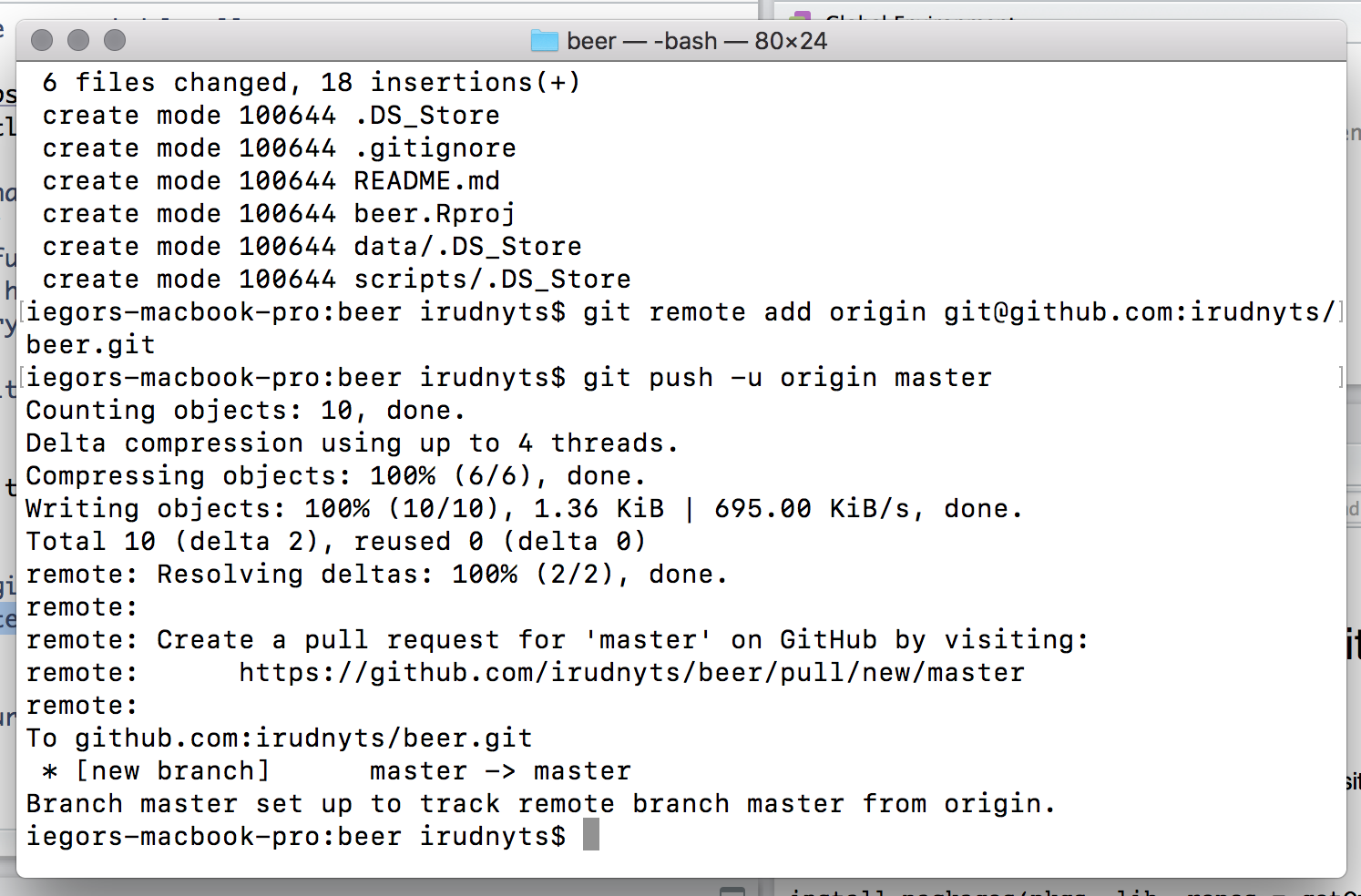
```
Refresh the page at your browser to ensure that changes appear at Github repo (do not freak out if you do not see all folders you have created, Git does not record empty folders).

Working with an existing data analysis project

Pull changes introduced by your collaborators by git pull.
Modify your files. If you want to delete a script, first off, move it to \depricated, and then remove it from there during the next iteration.
Add changes by git add --all and commit by git commit -m "A concious commit message.".
Push changes by git push. Merge changes if needed.