homework #3
Deadline: 2018-11-19 at 4pm
To submit your work, add samorso and irudnyts as collaborators to your private GitHub repo.
We will grade only the latest files prior to the deadline. Any ulterior modifications are pointless.
The objectives of this homework assignment are the followings:
- Become competent at programming effectively using if/else and iterations statements;
- Learn how to program effectively using functions and think like a programmer;
- Improve your collaborative skills via GitHub.
To begin with, create a (preferably private) GitHub repository for your group, and name it ptds2018hw3. Once again, make sure to add samorso and irudnyts as collaborators. This project must be done using GitHub and respect the following requirements:
- All members of the group must commit at least once.
- All commit messages must be reasonably clear and meaningful.
- Your GitHub repository must include at least one issue containing some form of TO DO list.
You can create one or several RMarkdown files to answer the following problems:
Problem 1: Finding $\pi$
In this problem, we consider a Monte-Carlo approach for approximating the value of $\pi$ (that you assume you do not know). To start with, let consider the square below, which has an area of 4, and let draw a circle inside of this square.
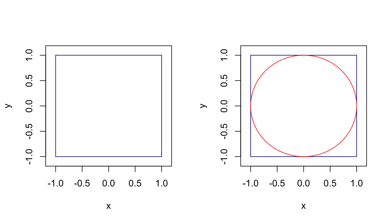 You can easily remark that this circle has a unit radius, and therefore its area is simply $\pi$. Indeed, remember that the area of a circle is $\pi r^2$ and in this case $r=1$.
Let us assume that the x and y coordinates are uniformly distributed between -1 and 1, that is $X\sim\mathcal{U}(-1,1)$ and $Y\sim\mathcal{U}(-1,1)$. We consider the following method for estimating the area of this circle:
1. Simulate $B$ coordinates $[X_i\;\;Y_i]^T$, $i=1,\dots,B$.
2. Create $Z$ a vector of Booleans, such that $Z_i = 1$ if $X_i^2 + Y_i^2 \leq 1$ and 0 otherwise.
3. Estimate $\pi$ as follows: $$\hat{\pi} = \text{area of the square } \times \frac{\text{number of points in the circle}}{\text{total number of points}} = 4 \frac{\sum_i^B Z_i}{B}.$$
If you want to understand why this method works, see the bottom of the page.
a) Create a function that approximates $\pi$ following the above recipe. Your function should be called find_pi() and should have three arguments:
B: the number of points for the approximation with defaults value = 5000,seed: a positive integer that controls the generation of random numbers with default value = 10,make_plot: a Boolean value that control whether or a not a graph should be made (see below for details and use FALSE as default).
Your function should look like:
find_pi <- function(B = 5000, seed = 10, make_plot = FALSE){
  # Control seed
  set.seed(seed)

  # Simulate B points
  point = matrix(runif(2*B, -1, 1), nrow = B, ncol = 2)

 ...

 return(hat_pi)
}
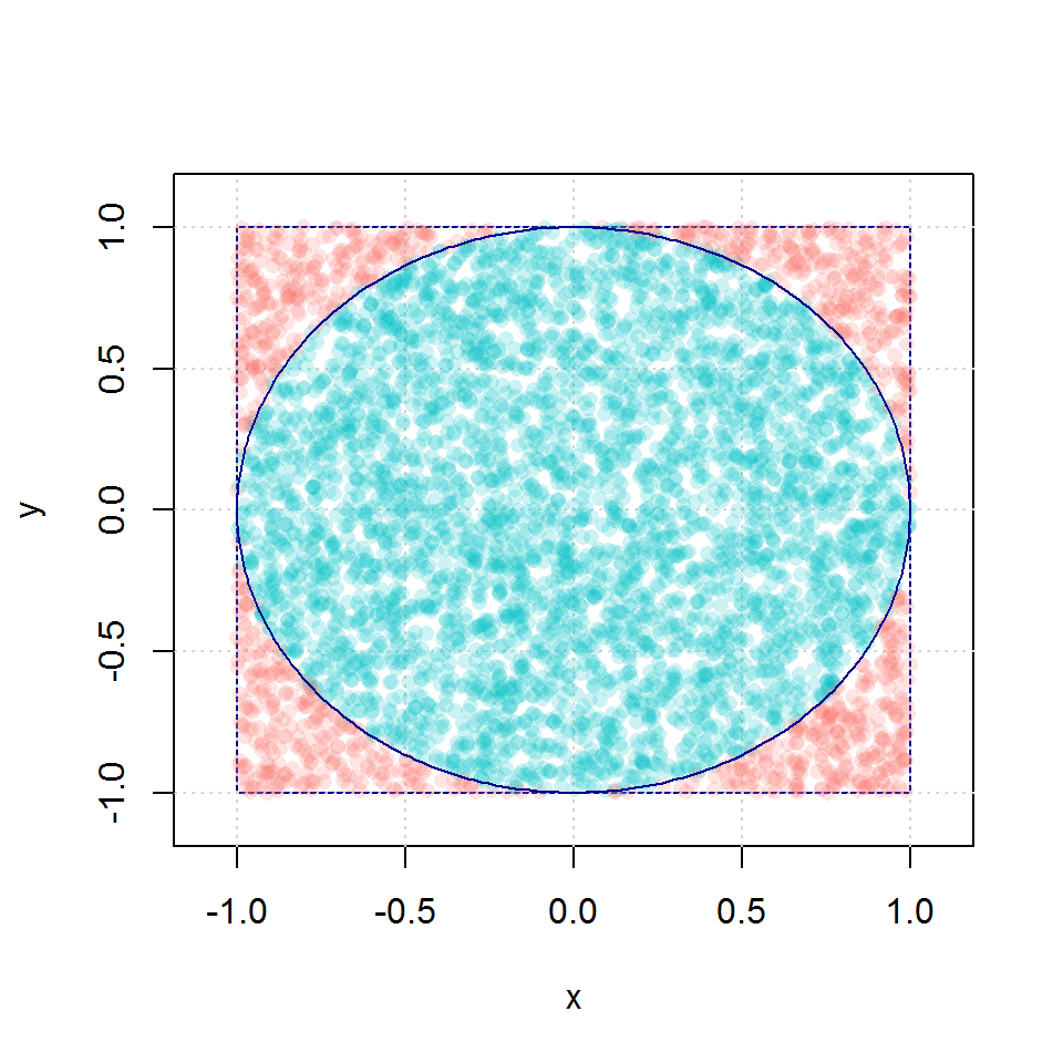
When enabling the plot by setting make_plot = TRUE, the function find_pi() should produce a graph with a square, a circle inside and the B points with two distinct colors according to whether the point is inside or outside the circle. See below for an example.
b) Verify that by running find_pi(B=10^8) the function returns the value 3.141747.
c) Evaluate the function with the values $B=100, 200, \dots, 10000$. Illustrate the obtained $\hat{\pi}$ and the true value of $\pi$.
Problem 2: Satellite Navigation System
Global Navigation Satellite Systems or GNSS are systems with global coverage that uses satellites to provide autonomous geo-spatial positioning. They allow small electronic receivers to determine their location (longitude, latitude, and altitude/elevation) to high precision (within a few meters) using time signals (i.e. “distances” informally speaking) transmitted along a line of sight by radio from satellites. Currently, there exist only three global operational GNSS, the United States’ Global Positioning System (GPS), Russia’s GLONASS and the European Union’s Galileo. However, China is in the process of expanding its regional BeiDou Navigation Satellite System into a global system by 2020. Other countries, such as India, France or Japan are in the process of developing regional and global systems.
Obviously, GNSS are very complex systems and in this exercise we will consider an extremely simplified setting to illustrate the basic concepts behind satellite positioning. If you are interested in learning more about GNSS, an excellent introduction to get started this topics can be found here: “An Introduction to GNSS”.
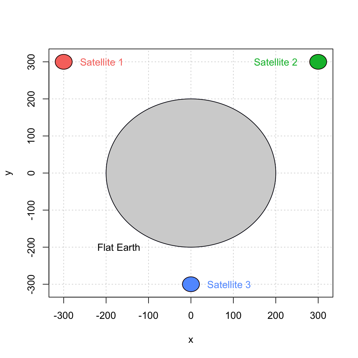
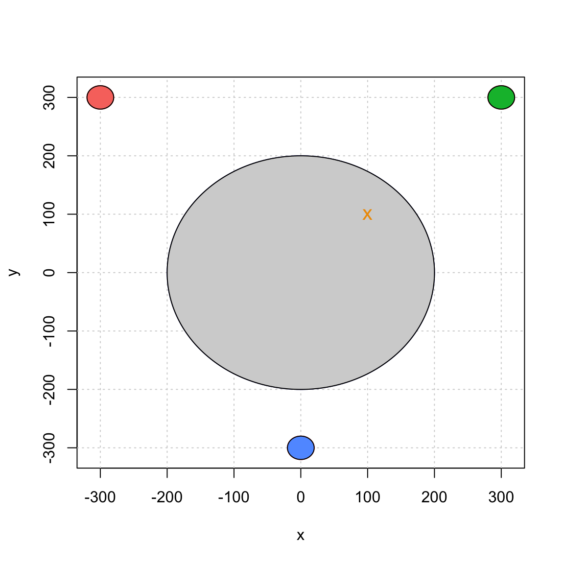
For simplicity, let us start by assuming that the earth is a motionless perfect circle in a two-dimensional space. Next, we assume that three motionless GNSS-like satellites are placed around the earth. The position of these satellites is assumed to be known and we will assume that there are synchronized (i.e. they all have the same “time”). Our simplified setting can be represented as follows:
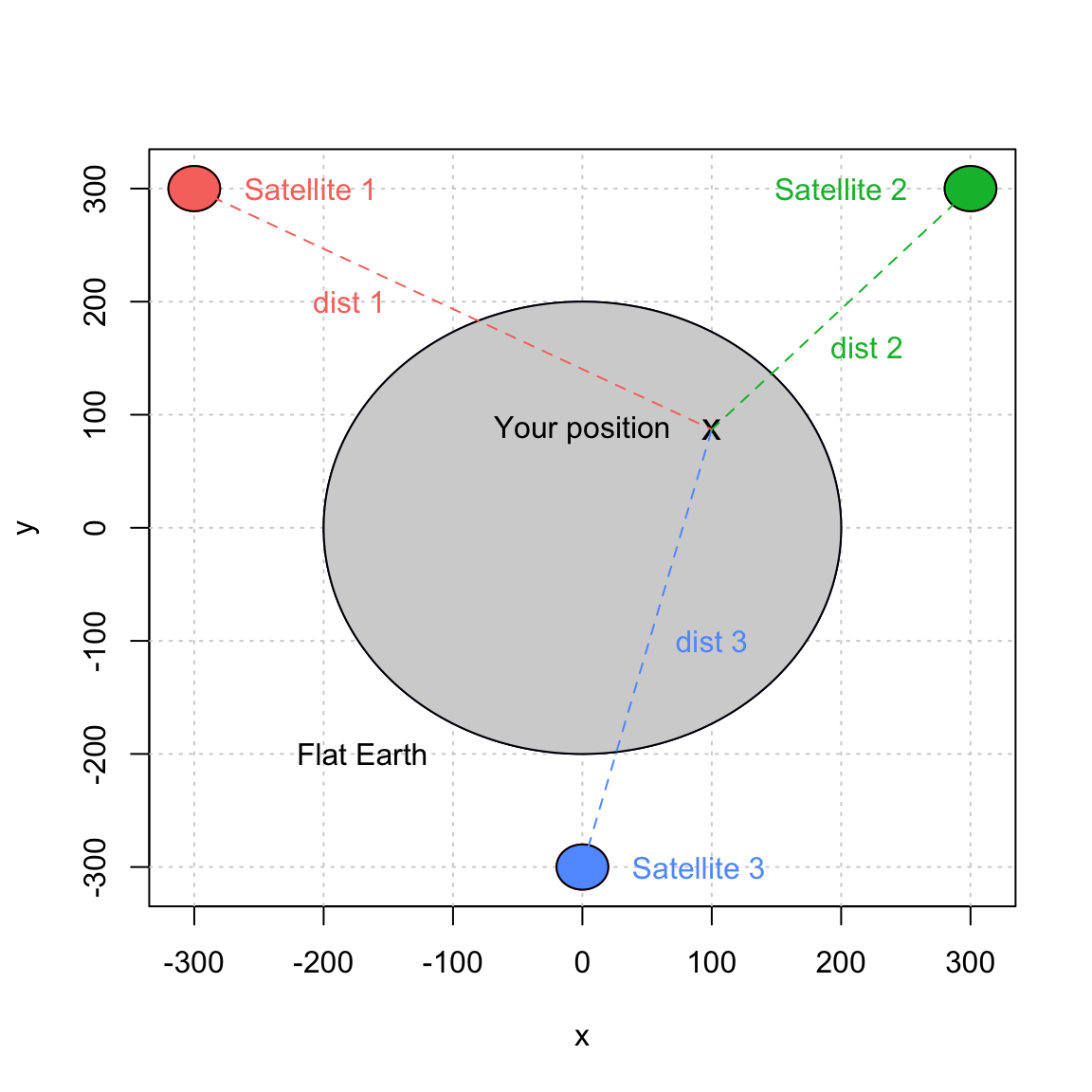
Now, suppose that you are somewhere on our flat earth with a GNSS-like receiver. The way you will be able to compute your position with such system is by first determining the distance (or a closely related notion) between yourself and with each satellite. The computation of these distances is done by comparing the time at which a signal is emitted by a satellite and the time at which it is received by your device. More precisely, let $t_e^{(i)}$ and $t_r^{(i)}$ denote, respectively, the times at which a signal is emitted and received for satellite $i$. To simplify further, we assume that $t_e^{(i)}$ (also known as the clock in each satellite) is “perfect” (this point may surprise you, but in reallity the time in the satellite are subjected to random variations). However, the clock in our device is not perfect and $t_r^{(i)}$ is estimated by $\hat{t}_r^{(i)}$ which represents the time recorded by the receiver device. Since all satellites are assumed to be synchronized, we can write $$\hat{t}_r^{(i)} = t_r^{(i)} + \Delta t,$$ where $\Delta t$ is the time difference, it is the same for all satellites as it does not depend on $i$. Using this simple result as well as the times $\hat{t}_r^{(i)}$ and ${t}_e^{(i)}$, we can compute the estimated distance between us and the $i$-th satellite as follows:$$ \hat{d}_i = c\left[(t_r^{(i)} + \Delta t) - t_e^{(i)}\right] = c\left(t_r^{(i)} - t_e^{(i)}\right) + c \Delta t = d_i + \varepsilon,$$ where $c$, $d_i$ and $\varepsilon$ denote, respectively, the speed of the signal, the true distance between us and the $i$-th satellite, and the measurement error. This setting can be represented as follows:
 Next, we let $(x_i, y_i), \, i = 1,2,3$ denote the position of satellite $i$. The coordinates of these points are given in the table below:
| $i$ | $x_i$ | $y_i$ |
|---|---|---|
| 1 | -300 | 300 |
| 2 | 300 | 300 |
| 3 | 0 | -300 |
Finally, we let $(x_0, y_0)$ denotes our position on earth. Then, the distance between our position and the $i$-th satellite is given by $$ d_i = \sqrt{\left(x_i - x_0\right)^2 + \left(y_i - y_0\right)^2}. $$ Unfortunately, $d_i$ is unknown (if our position were known, why using a GNSS system). Instead, we can express the distance as $d_i = \hat{d}_i - \varepsilon$. We obtain following system of equations: $$ \begin{aligned} (x_1 - x_0)^2 + (y_1 - y_0)^2 &= (\hat{d}_1 - \varepsilon)^2 \\ (x_2 - x_0)^2 + (y_2 - y_0)^2 &= (\hat{d}_2 - \varepsilon)^2 \\ (x_3 - x_0)^2 + (y_3 - y_0)^2 &= (\hat{d}_3 - \varepsilon)^2, \end{aligned} $$ where $\boldsymbol{\theta}=[x_0\;\;y_0\;\;\varepsilon]^T$ are the three unknown quantities we wish to estimate and $\hat{d}_i,\;i=1,2,3,$ are the observations.
While there exists several methods to solve such estimation problem, the most common is known as the “least-square adjustement” and will be used in this problem. It is given by: $$ \hat{\boldsymbol{\theta}} = \operatorname{argmin}_{\boldsymbol{\theta}} \; \sum_1^3 \; \left[\left(x_i - x_0\right)^2 + \left(y_i - y_0\right)^2 - \left(\hat{d}_i - \varepsilon\right)^2\right]^2. $$
a) Write a general function named get_position() that takes as a single argument a vector of observed distances and returns an object with an appropriate class having custom summary and plot functions. For example, suppose we observe the vector of distances $$ \hat{\mathbf{d}} = [\hat{d}_1\;\;\hat{d}_2\;\;\hat{d}_3]^T = [449.2136\;\;284.8427\;\;414.3106]^T, $$ then you should replicate (approximately) the following results:
position = get_position(c(453.2136, 288.8427, 418.3106))
summary(position)
## The estimated position is:
## X = 99.9958
## Y = 100.003
plot(position)
Note that inside the get_position() function, you need to estimate the positions $\hat{x}$ and $\hat{y}$. You can use the R function optim for this purpose. It has the syntax:
optim(par = starting_values, fn = my_objective_function, arg1 = arg1, ..., argN = argN)
The arguments are:
- starting_values: the starting values for the optimization, here a vector of three values corresponding to $\hat{\boldsymbol{\theta}}$.
- my_objective_function: the objective function, here the one we defined above. It must have $\boldsymbol\theta$ as one of its arguments.
- arg1 to argN: additional arguments for the objective functions.
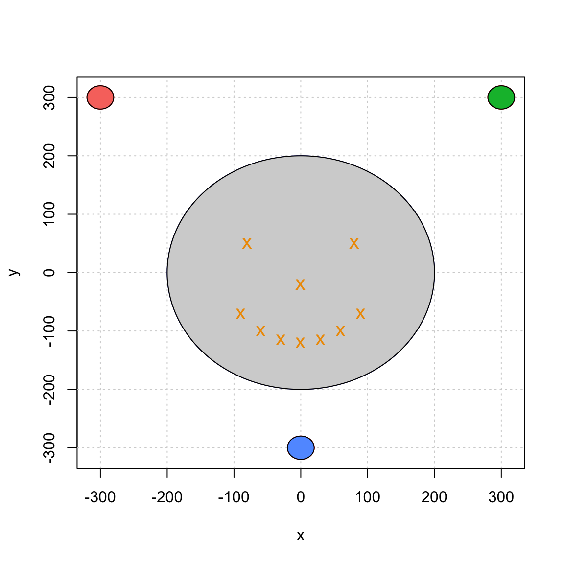
b) Generalize the function get_position() of the point a) to accept also a matrix of observed distances (but keep only one argument!).
c) Verify that the function you wrote at the point b) display the same graph
position = get_position(dist_mat)
summary(position)
where the matrix inputed is
##           [,1]     [,2]     [,3]
##  [1,] 458.9474 337.1013 363.1112
##  [2,] 337.0894 458.9355 363.0993
##  [3,] 442.5835 442.5835 283.9493
##  [4,] 520.1845 520.1845 184.0449
##  [5,] 534.1411 499.0299 191.3455
##  [6,] 499.1322 534.2434 191.4479
##  [7,] 542.0904 470.4216 212.7515
##  [8,] 470.4070 542.0758 212.7369
##  [9,] 541.6032 429.4569 250.9978
## [10,] 429.4120 541.5583 250.9528
Technical explanations around problem 1
To understand why the method presented works, let us show that $$\mathbb{E}\left[\hat{\pi}\right] = \pi.$$ To prove this result, we start by noticing that $f(x,y) = f_X (x) f_Y (y) = 1 / 4$ if $x\in[-1,1]$ and $y\in[-1,1]$ and 0 otherwise.
Let $Z_i = 1$ if $X_i^2 + Y_i^2 \leq 1$ and 0 otherwise. Let $A$ be the space such that $x^2+y^2\leq1$. Then, we obtain $$ \begin{aligned}\mathbb{E}\left[Z_i\right] &= \iint_A f(x,y) dx dy = \frac{1}{4} \iint_A dx dy \\ &= \frac{1}{4} \int_0^1 \left[\int_0^{2\pi} r d\theta\right] dr = \frac{\pi}{2} \int_0^1 r dr = \frac{\pi}{4}.\end{aligned}$$ Therefore, we have $$ \mathbb{E}\left[\hat{\pi}\right] = \mathbb{E}\left[4 \frac{\sum_i^B Z_i}{B}\right] =4 \mathbb{E}\left[Z_i\right]= 4 \frac{\pi}{4} = \pi.$$
If you want to know more about of $X^2 + Y^2$ (i.e. the sum of independent squared uniform random variable), which has a really surprising distribution, here is an interesting article: “Sum of squares of uniform random variables” by Ishay Weissman.