homework #2
Deadline: 2018-11-05 at 4pm
To submit your work, add samorso and irudnyts as collaborators to your private GitHub repo.
We will grade only the latest files prior to the deadline. Any ulterior modifications are pointless.
The objectives of this homework assignment are the followings:
- Learn how program effectively using if/else and iterations statements;
- Become familiar with using data frame objects and mapping packages;
- Constructing a portfolio;
- Become familiar with GitHub and using it as a collaborative tool.
To begin with, create a (preferably private) GitHub repository for your group, and name it ptds2018hw2. Once again, make sure to add samorso and irudnyts as collaborators. This project must be done using GitHub and respect the following requirements:
- All members of the group must commit at least once.
- All commit messages must be reasonably clear and meaningful.
- Your GitHub repository must include at least one issue containing some form of TO DO list.
You can create one or several RMarkdown files to answer the following problems:
Problem 1: Fizz Buzz
Write a program that prints the numbers from 1 to 1000, but with the following specific requirement:
- for multiples of three, print “Fizz” instead of the number;
- for the multiples of five print “Buzz” instead of the number;
- for numbers which are multiples of both three and five print “FizzBuzz” instead of the number.
An example of the output would be:
1, 2, Fizz, 4, Buzz, Fizz, 7, 8, Fizz, Buzz, 11, Fizz, 13, 14, FizzBuzz, 16, 17, Fizz, 19, Buzz, Fizz, 22, 23, Fizz, Buzz, 26, Fizz, 28, 29, FizzBuzz, 31, 32, Fizz, 34, Buzz, Fizz, ...
Problem 2: Map
Using the same tools we used in class, create a simple map to represent the volume of the real estate market in Switzerland. More specifically, the goal of this problem is to reproduce as closely as possible the map below:
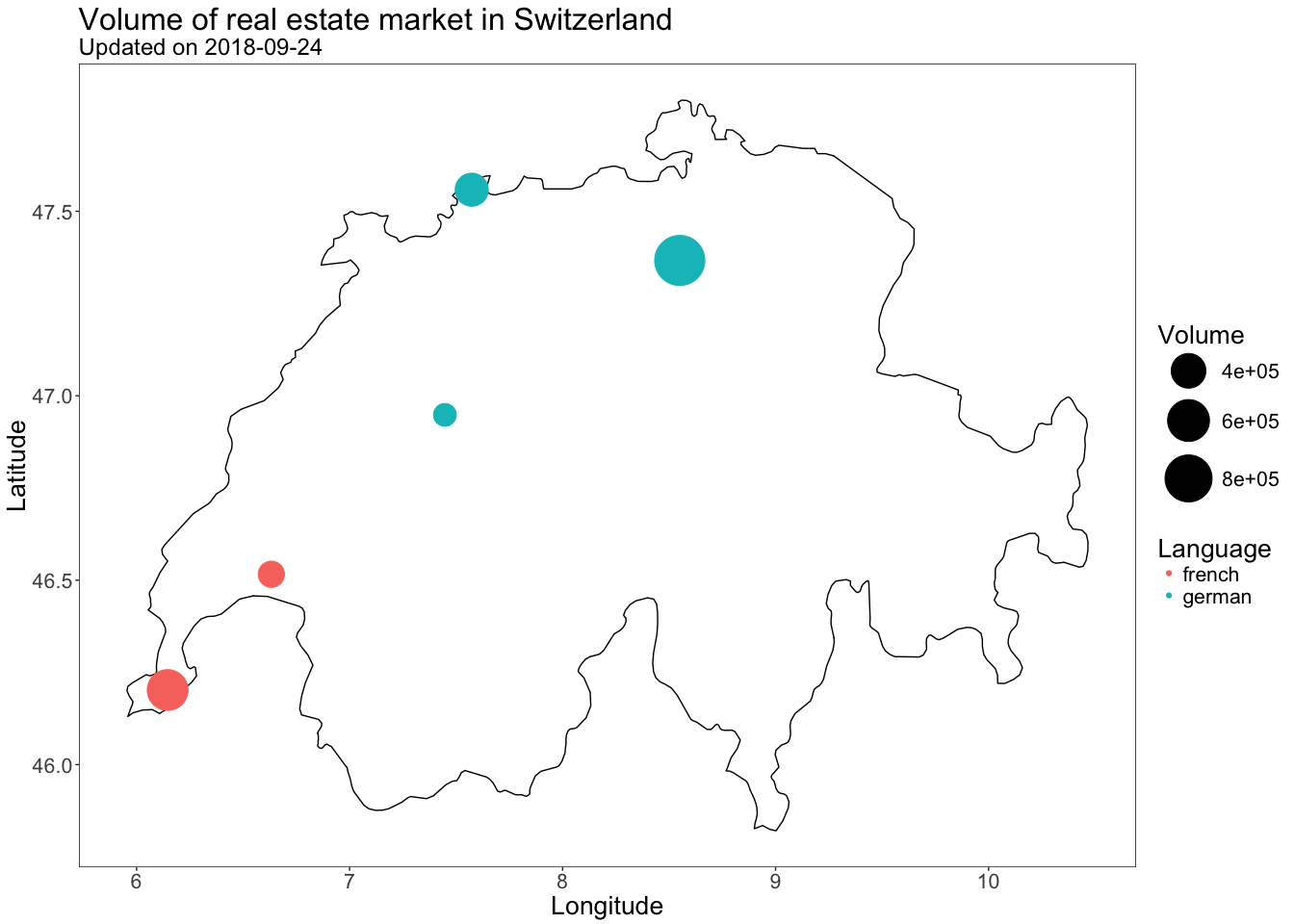
Note that the code below was used to scrap the data needed for this graph:
# Please do not forget to update ptds2018

library("rworldmap")
library("rworldxtra")
library("ggmap")
library("tidyverse")
library("magrittr")
library("ptds2018")

cities <- data.frame(
    name = c("zurich", "bern", "lausanne", "geneva", "basel"),
    language = c("german", "german", "french", "french", "german"),
    stringsAsFactors = FALSE
)

# Scrap prices from comparis.ch
#-------------------------------------------------------------------------------

volumes <- sapply(cities$name, get_volume)

cities <- cbind(
    cities,
    data.frame(volume = volumes)
)

# ...or use dplyr
# cities <- cities %>%
#     dplyr::mutate(volume = volumes)

# Define cities' coordinates
#-------------------------------------------------------------------------------

cities <- cbind(
    cities,
    geocode(location = cities$name, source = "dsk")
)


# Draw the map
#-------------------------------------------------------------------------------

world_map <- getMap(resolution = "high")

which(sapply(1:243, function(x) world_map@polygons[[x]]@ID) == "Switzerland")

switzerland <- world_map@polygons[[40]]@Polygons[[1]]@coords %>% as_tibble()

# your code goes here
Problem 3: 3D-random walk
In this problem you will program a three-dimensional random walk. For this purpose we will consider a three-dimensional space where we let $\mathbf{X}_0 = [0 \;\; 0\;\; 0]^T$ denote the starting point of our process. Suppose that there exists a sequence of (univariate) random variables $U_1, \cdots, U_B$ such $U_t \stackrel{iid}{\sim} \mathcal{U}(0,1)$. Then, we let the position at time $t$ (where $1 \leq t \leq B$) be given by $$\mathbf{X}_t = \mathbf{X}_s + \mathbf{f}(U_t),$$ where $s=t-1$. The function $\mathbf{f}$ gives the new direction. For simplicity, we assume that at each time $t$ the process moves one-step forward or backward in (only) one of the three dimensions. Let us introduces five “threeshold values” $0\leq a_1<a_2<a_3<a_4<a_5\leq1$. So to be concrete, the function $\mathbf{f}$ returns the following vectors:
- $[+1\;\;0\;\;0]^T$ if $U_t\leq a_1$,
- $[-1\;\;0\;\;0]^T$ if $U_t\in(a_1,a_2]$,
- $[0\;\;+1\;\;0]^T$ if $U_t\in(a_2,a_3]$,
- $[0\;\;-1\;\;0]^T$ if $U_t\in(a_3,a_4]$,
- $[0\;\;0\;\;+1]^T$ if $U_t\in(a_4,a_5]$,
- $[0\;\;0\;\;-1]^T$ if $U_t>a_5$.
For example, let $B = 2$, $a_i = \frac{i}{6}$, $U_1 = 0.12$ and $U_2 = 0.81$ then we have, at the first step, $$ \mathbf{X}_1 = \mathbf{X}_0 + \mathbf{f}(U_1) = [0\;\;0\;\;0]^T + [1\;\;0\;\;0]^T = [1\;\;0\;\;0]^T, $$ and at the second step, $$ \mathbf{X}_2 = \mathbf{X}_1 + \mathbf{f}(U_2) = [1\;\;0\;\;0]^T + [0\;\;0\;\;1]^T = [1\;\;0\;\;1]^T. $$
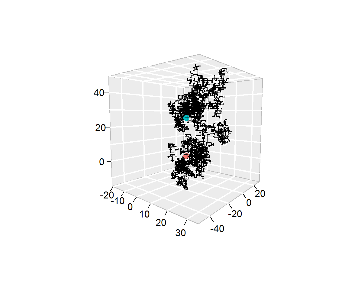
- (a) Using the same idea, simulate a three-dimensional random walk with $B = 10^4$, $a_i = \frac{i}{6}$ and with $U_t$ being obtained as follows:
B <- 10^4
set.seed(1982)
Ut <- runif(B)
Notice that $U_t$ corresponds to the t-th element of Ut. With this configuration, show that a the last step you obtain $$ \mathbf{X}_B = [26\;\;-44\;\;26]^T, $$ and provide a graphical respresentation of your random walk. For example, you can produce a graph similar to the one below which is based on the function segments3D from the plot3D package. Note that the red and blue points indicate, respectively the starting and end points of the random walk.
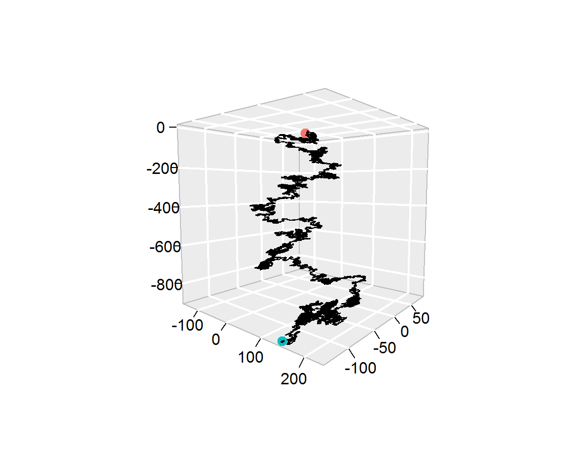
- (b) Repeat part (a) by modifying the parameters: $B = 10^5$, $a_i = 0.99 \frac{i}{6}$ and with $U_t$ being obtained as follows
B <- 10^5
set.seed(2000)
Ut <- runif(B)
Verify that you obtain $$ \mathbf{X}_B = [142\;\;-133\;\;-899]^T $$ and produce a graph similar to:
- bonus Use the package
animationto create a video that shows how a random walk evolves over time.
Problem 4: portfolio construction
Suppose that you are working in an investment firm company as a quantitative analyst. Your boss gives you the task of creating a portfolio for one of your clients. The client wants to find the portfolio with the smallest variance that satisfies the following constraints:
- Invest exactly $1,000,000.
- Only invest in stocks that are in the S&P500 index.
- Spend less than $100 in execution.
Your execution fees (i.e. the cost of buying shares) are given by $C_i = \max \left(\$40, \$ 0.0001 \cdot X_i \right)$ for each transaction where $X_i$ represent the amount of money you wish to invest in stock $i$. For example, if you want to invest 30% and 70% in stocks A and B your total cost would be $$ \text{Cost} = C_1 + C_2 = \max \left(\$40, \$ 0.0001 \cdot 0.3 \cdot 10^6 \right) + \max \left(\$40, \$ 0.0001 \cdot 0.7 \cdot 10^6 \right) = \$40 + \$70 = \$110. $$
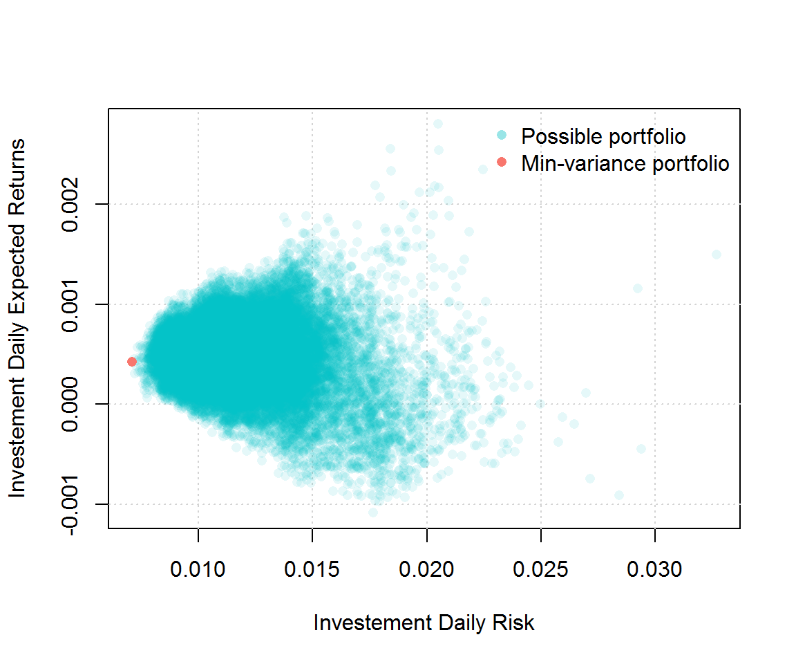
Note that $\sum_i X_i = \$1,000,000$. Therefore, your boss requires that you compute all possible portfolios that satify the client’s constraints, represent them graphically as (for example) in the graph below and find the weight of the best (i.e. minimum variance) portfolio.
In order to complete this task, your boss tells you to use 3 years of historical data and gives you this code to download the data you will need (how kind of him/her):
library(quantmod)
library(rvest)
sp500 <- read_html("https://en.wikipedia.org/wiki/List_of_S%26P_500_companies")

sp500 %>%
html_nodes(".text") %>%
html_text() -> ticker_sp500

SP500_symbol <- ticker_sp500[(1:499)*2+1]
SP500_symbol[SP500_symbol == "BRK.B"] <- "BRK-B"
SP500_symbol[SP500_symbol == "BF.B"] <- "BF-B"
Your boss also mentions that the function get() could be useful for this project and provides you with the example below (what a really nice boss!):
library(quantmod)
today <- Sys.Date()
three_year_ago <- seq(today, length = 2, by = "-3 year")[2]
stocks_tickers <- c("AAPL", "MSFT")
getSymbols(stocks_tickers, from = three_year_ago, to = today)
nb_ticker <- length(stocks_tickers)
var_stocks <- rep(NA, nb_ticker)
names(var_stocks) <- stocks_tickers

for (i in 1:nb_ticker){
Xt = na.omit(ClCl(get(stocks_tickers[i])))
stocks_tickers[i] = var(Xt)
}
stocks_tickers